Part 2: The Perceptron

The ancestor of today’s machine learning models was invented in the late 1950s by Frank Rosenblatt, and was named ‘The Perceptron’.

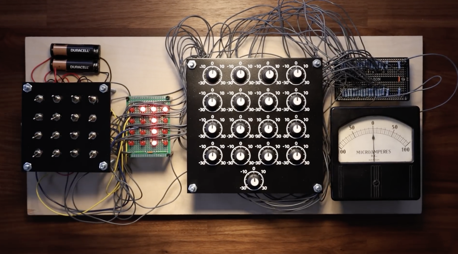
It’s possible to build out a perceptron very simply, and they are a wonderfully manual, tactile way to develop an understanding of how machine learning works at its core. Today’s most advanced Large Language Models are essentially built out of millions of the modern equivalent of a perceptron.

The perceptron, while brilliant, had a critical flaw. When this was recognised, it led to the first ‘AI Winter’ in the mid 1970s. We will discuss how this was overcome in the next chapter.

Let’s build out a perceptron ourselves so we can understand the roots of everything that was to follow.

Classification

The problem that the Perceptron aimed to solve was slightly different from the one our linear model solved: how to classify things.

For example, how can we train a model to tell if an image is of a cat or a dog? Or to analyse handwriting? We will do this more rigorously later, when we tackle convolutional neural networks and diffusion, but for now, let’s consider a simplified problem.

Let’s imagine we need to train a model to tell the difference between the character L and the character T.

Let’s use 4x4 ‘images’ of these characters, for example:

T

L

T

L

T

L

…and so on.

This is no longer a line of best fit problem, per se: it’s a classification problem. We want to know: what class is the image - an L or a T?

Each of the 16 pixels can be ‘on’ or ‘off’. So at its heart, this problem is about deciding whether each pixel being ‘on’ or ‘off’ makes it more or less likely to be a T or an L.

We can use straight lines to do this, but rather than plotting a line of best fit between continuous data points as with our linear model, the lines will form a boundary between the two classes. If a sample falls on one side of the line, it’s more likely to be a T; on the other, an L.

This line is called the decision boundary.

The Decision Boundary

We can’t easily draw a chart with more than two dimensions ( $x$ and $y$ ), and we clearly need 4x4 = 16 dimensions to capture the on/off state of all 16 pixels.

However, we can illustrate the idea of the decision boundary by taking a 2D sample of the data. We can take a row and a column for $x$ and $y$ , and then plot their values for a single T and a single L.

T

L

Notice:

the top row (all ‘on’ in the T, only one ‘on’ in the L)

T

L

the left column (all ‘on’ in the L, only one ‘on’ in the T)

T

L

If we add up the values for the row and the column (using ‘on’ = 1, ‘off’ = 0) for the two samples, we get:

	Top row ( $x$ )	Left column ( $y$ )
`T`	1+1+1+1 = 4	1+0+0+0 = 1
`L`	1+0+0+0 = 1	1+1+1+1 = 4

Now we can plot the chart - see below.

You’ll see the values for the T cluster at $[4, 1]$ , and the values for L cluster in the opposite corner, at $[1,4]$ .

We can then cleanly separate the T and the L with a straight line to form our decision boundary.

T: (4, 1)L: (1, 4)

Show decision boundary

Now we know that if a new sample’s top row sums to around 4, it’s more likely to be a T, and if its left column sums to 4, it’s more likely to be an L.

We can go further than this and say that if the value for $x$ (the top row) is greater than 1, it’s likely to be a T, and if the value for $y$ (the left column) is greater than 1, it’s likely to be an L.

This example shows a 2-dimensional ‘slice’ of the full 16-dimensional dataset, illustrating what the decision boundary does. Now it’s just a question of scaling up the dimensions. Conceptually, you can understand:

In 2D, the decision boundary is a line
In 3D it becomes a plane (like a 2D sheet through the $x$ , $y$ and $z$ space)
In higher dimensions, it becomes a ‘hyperplane’, which is impossible to visualise.

However, the point is: the boundary is straight and it cuts between the feature clusters. The maths for a straight line will work.

So far, so good. We can still use the straight line equation, $y=mx+c$ (or $w·x + b$ using weights and a bias), for the decision boundary. This will generate a number that represents a score — how likely the input was to belong to one class or the other. However, we have a couple of adjustments that we need to make to get the equation working for our use-case.

Multiple inputs

Our model needs to capture whether each of the 16 pixels is on or off in a given sample. This is clearly not something we can model with a single input value for $x$ as with our previous model — we need an input for each pixel.

That means the input, $x$ , for our model is now an array. The output (prediction), $y$ , will be a binary (0 or 1) indicating whether the input is of class T or class L:

// Our 'T' from above, expressed as an array
const input = [
  1, 1, 1, 1,
  0, 1, 0, 0,
  0, 1, 0, 0,
  0, 1, 0, 0,
]
// X is a 1x16 array
// the Y returned is 0 or 1
perceptron.predict(input), // e.g. 1 for T

How do we do this?

If $x$ is now an array of values, then we can scale our $y=mx+c$ (or y = weight * x + bias) by adding a weight for each value of $x$ .

Since we have 16 values for $x$ , we need 16 weights:

let w = [...// 16 weights]
let b = 0.5 // Bias

// Our input
let x = [...// 16 values]

// Calculate y = wx + b
let wx = (w[0] * x[0]) + (w[1] * x[1]) + (w[2] * x[2]) // ...all 16 
let y = wx + b

Sigma, dot products and weighted sums

We are aiming to build our mathematical intuition from the ground up. The goal is to be able to pick our way through the equations in ML papers and get a sense of how models work out in the wild.

As part of this, we will introduce symbols and principles as we go. Some new ideas that will help us at this stage are:

Sigma, $Σ$ - the Greek upper-case ‘S’, which means ‘sum’. It’s used to describe a loop that adds things up.
As an example, adding w[i] * x[i] for 16 weights and inputs can be written like this:

$\sum_{i=0}^{15} w_i x_i$

Note that we are essentially showing:

let sum = 0
for(let i=0; i<16;i++) sum += w[i] * x[i]

Dot product - in mathematics, a ‘product’ is the value of something multiplied by something else, like A*B. ‘Dot product’ is the name for multiplying several corresponding items (w and x here), and then adding them up to produce one value. It’s simply written as a dot ( $⋅$ ).

So $\sum_{i=0}^{15} w_i x_i$ can be written more generally as $w⋅x$ . The former specifies the number of items we are summing (i = 0 to 15) and captures the idea of a loop; the latter says we are summing all the products of our ws and xs, however many there are.

Weighted sum - This is the term given to $w⋅x + b$ (i.e., adding the bias to the dot product of all the ws and all the xs). So our output for $y$ is the weighted sum of $w⋅x + b$ .

Let’s sketch this out in code:

function perceptron(dimensions) {
  let weights = Array(dimensions).fill(0)
  let bias = 0

  return {
    // x is an array of 16 pixels 
    predict(x) {
      let dotProduct = 0
      for (let i = 0; i < dimensions; i++) {
        // multiply each x pixel by its weight
        // and add it to the sum
        dotProduct += weights[i] * x[i];
      }
      // add the bias to get the weighted sum
      let y = dotProduct + bias;
      return y
    }
  }
}

const t = [
  1,1,1,1, 
  0,1,0,0, 
  0,1,0,0, 
  0,1,0,0
]
const prediction = perceptron.predict(t) // outputs weighted sum

So now,

The predict method will take an input array of the 16 pixels
we will map each pixel to a corresponding weight,
multiply each pixel by its weight ( $wx$ for each one),
add all these $wx$ products together to get the dot product
add the bias at the end to get the weighted sum

The symbols and terminology muddy the waters a bit, but hopefully the underlying method here is not too hard to grasp.

Now we are only missing one piece: how to convert our weighted sum into binary classification.

Thresholds

Our model is for classifying whether an input is a T or an L, which is a binary output (i.e. one or the other). But as-is, our weighted sum will be a number like 4.7 or -2.5, which won’t work.

So we need to somehow normalise our output so that it is a binary.

The way we do this is to add a threshold:

let dotProduct = ...
let weightedSum = dotProduct + bias // some number, like 4.2

return weightedSum > threshold ? 1 : 0

So what is threshold?

In ML, this is handled through some sort of activation function that takes the raw weighted sum and turns it into something useful (we will come back to this in the next chapter). In the perceptron, the activation function was a simple step function:

/**
 * The step function turns a number into a binary output
 */
function step(x) {
  // In the step function, the threshold can just be 0
  return x > 0 ? 1 : 0
}

So if the weighted sum is a negative number, whatever it is, it will output 0. If it’s a positive, it will output 1.

This simple binary output means we don’t even need gradient descent to train this model (in fact, gradient descent came later). This is because the binary output is either correct or incorrect, so we can nudge the weights directly.

So, for every pixel that was ‘on’ in this input, we just increase or decrease its corresponding weight depending on whether it was correct or incorrect. This will change its effect on the output.

If a pixel has a large bearing on the outcome (e.g. if the top right pixel is ‘on’, it’s almost certainly a T), then it can have a more significant weight.

// In the training loop
const prediction = model.predict(x)

// Learning without gradient descent:
if(prediction !== actual) {
  if(actual === 1) {
    // should have output 1, so we need 
    // to make the weighted sum bigger
    // for this specific input pattern
    weights = weights.map((w, i) => w + x[i])
  } else {
    // should have been 0, make the 
    // weighted sum smaller for this
    // specific pattern
    weights = weights.map((w, i) => w - x[i])
  }
}

If the end output should be higher, we want pixels that are “on” (1) to have more positive influence, so we increase their weights. If output should be lower, we decrease them.

Manual training

Training Rosenblatt’s original hardware perceptron was a very manual process, and dialling the weights in yourself is a great way to build an intuition for how the model works.

Try the manual perceptron trainer below. You’re doing the same update rule as the code, just by hand.

The goal is to get the perceptron to output 1 for T and 0 for L. Here are the steps to the algorithm:

Load a T pattern (or create one) and adjust weights until the output is 1
Next, load an L pattern (or create one) - does it still work? Again, adjust weights if needed until the output is 0.
Keep iterating until both patterns are classified correctly

Manual Perceptron Trainer

Input (click to draw)

→

Weights (click to select)

→

Output

Σ = 0.00

Click a weight cell to adjust it

Bias:+0.0

You will notice a couple of things:

You need very few ‘training loops’ to build a pretty robust model
You will likely end up with positive weights in the top row (where Ts tend to have pixels) and negative weights in the bottom row and left column (where Ls usually have pixels).

Implementing the Perceptron

We’ve got everything we need to build out a perceptron now, and we have also developed a grip on the maths behind the model, which will stand us in good stead as we move on to more advanced ideas.

Any model is only as good as its data, so let’s start there. We will use 10 samples of each class. We will include samples with ‘noise’ (random pixels) and missing pixels, which will help our model to generalise well.

10 4x4 images of Ts and Ls

import { data } from './data.js';

function perceptron(dimensions) {
  let weights = Array(dimensions).fill(0);
  let bias = 0;

  return {
    predict(x) {
      let dotProduct = 0;
      for (let i = 0; i < dimensions; i++) {
        dotProduct += weights[i] * x[i];
      }
      // Step activation
      return (dotProduct + bias) > 0 ? 1 : 0;
    },
    // Perceptron update rule (no gradients needed)
    update(x, delta) {
      for (let i = 0; i < dimensions; i++) {
        weights[i] += delta * x[i];
      }
      bias += delta;
    },
  };
}

function train(hyperparams, getModel, data) {
  const { epochs } = hyperparams;
  const dimensions = data[0].pixels.length;
  const model = getModel(dimensions);

  for (let epoch = 0; epoch < epochs; epoch++) {
    let errors = 0;

    for (const { pixels: x, label: actual } of data) {
      const predicted = model.predict(x);

      // "Loss" for perceptron: just right or wrong
      if (predicted !== actual) {
        const delta = actual - predicted; // +1 or -1
        model.update(x, delta);
        errors++;
      }
    }

    console.log({ epoch, errors });
    if (errors === 0) break;
  }

  return model;
}

const model = train({ epochs: 10 }, perceptron, data);

Notes on the code

As we move on to more complex models, it’s worth reinforcing some ideas here.

No gradient descent

The perceptron predates backpropagation and uses a simpler update rule — if wrong, nudge weights directly by adding or subtracting the input values. You can probably sense that this won’t scale well.

Simpler hyperparameters

No learning rate (implicitly 1, since we nudge the weights by 1 or -1), no normalization (inputs are already 0/1), no MSE loss (just right or wrong). We only need epochs. You saw in the previous chapter that for any level of complexity, hyperparameters are key.

Converges fast

Because the problem is linearly separable and the update rule is direct, we typically hit zero errors within a handful of epochs.

Initialisation is deterministic

With this code, the weights would be identical after every run, but that’s because the initialisation is deterministic (all zeros) and the data is the same.

However, there are infinitely many valid decision boundaries for linearly separable data like ours. You might have found with the manual trainer above that there were multiple valid solutions.

Below are several training runs using this code, and data, but I shuffled the data each time. You could also generate more examples by initialising the weights to random floats like we did with our linear regression model.

Run 1

+1

+1

+2

+1

-1

+1

+0

+0

-1

+1

+0

+0

-1

+0

-2

-2

Run 2

+2

+1

+2

+2

-1

+0

+1

+0

-1

+0

+1

+0

-1

-2

-1

-1

Run 3

+0

+1

+1

+1

+0

+0

+0

+0

-1

+1

+0

+0

-1

+0

-1

-1

You can see that the model finds a solution, not the solution. As we build more complex models, we can use this principle of non-deterministic initialisation to make them more robust.

Summary

We’ve built a perceptron from scratch and learned the core mechanics that underpin modern ML:

Weighted sums: multiplying inputs by weights and adding a bias ( $w \cdot x + b$ )
Activation functions: converting raw outputs into something useful (here, a step function)
Decision boundaries: straight lines (or hyperplanes) that separate classes

The perceptron works well for problems where a straight line can cleanly divide the classes — problems that are linearly separable.

But what happens when a straight line isn’t enough? In the next chapter, we’ll hit the perceptron’s fatal limitation and see how stacking perceptrons into layers finally cracked the problem.